Raster Modeling

Objectives

The goal of this lab was to utilize various raster geoprocessing tools to build models to find sand mining suitability and risks to the environment and community of Trempealaeu County, WI. This was done in three parts: First, I must create a suitability model from newly created spatial layers for mining criteria such as geology, land use cover, distance to roads, slope, and water depth. This model will show prime locations for sand mining. Second, I need to create a risk model mapping the potential environmental and community impacts from sand mining. Lastly, I must overlay the two models to determine the best locations for sand mines in Trempealaeu County, WI. in which optimal conditions for sand mining and minimal environmental and community risk met.

Data sets used in this lab come from the Trempealeau County Land Records Division Website and from the National Land Cover Dataset gathered from the NLCD website.

Methods

There are three sections of this lab in which I 1. create a suitability model for stuitable mining land, 2. create a risk model for mapping potential impacts to the environment and community, and 3. Combine the models to determine the best locations for sand mines.

To create the suitability model, I first created several spatial layers. The first of these layers was geology. In Wisconsin, the Cambrian Jordan (Ej) and Wonewoc (Ew) sandstone types are the most ideal frac sands because of their grain size and sorting. Therefore, after converting the geology feature class into a raster using the Feature To Raster conversion tool, I reclassed the raster values to rank these layers as most important (Table 1) (Fig. 1). All feature classes for all spatial layers were projected into the NAD 1983 Wisconsin (US Feet) coordinate system  and clipped to the study area within Trempealeau County before any other tools were run.

Fig. 1: ModelBuilder process for creating the geology spatial layer.

Table 1: Reclassification of values for spatial layers used to build the Suitability Model.

3 is most important, 0 is excluded.

A landcover spatial layer was created using NLCD2011 features. I used the Polygon to Raster conversion tool to create a raster that would give me values showing type of land cover. I then reclassed the values twice: once for most suitable land cover types and another for excluding land cover types completely incapable of housing sand mines (Fig. 2). For the first reclassification, I deemed Hay/Pasture and Herbaceauous as "most important," or most suitable for mining as this land is not developed and requires little clearing for building a mine in the area. Values classified as "2" were landcover types that were not developed but required some clearing before a mine could be built. Landcover types reclassed as a 1 were areas of development, areas requiring significant clearing before building, and areas completely unsuitable for mining such as areas containing water. The exclusion reclassification excluded all areas containing water and developed areas having relatively high percentages of urban or residential development (Table 1).

Fig. 2: ModelBuilder process for creating reclassified landcover layers.

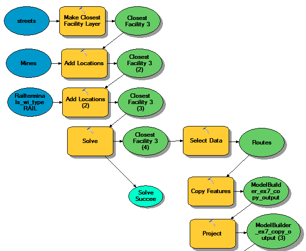
Proximity to rail terminals was found by utilizing the Euclidean Distance tool. Then, the resulting values from the Euclidean Distance output was reclassified to show higher suitability in areas closer to terminals than farther (Table 1) (Fig. 3).

Fig. 3: ModelBuilder process for creating spatial layer with distance from rail terminals.

Slopes can effect the suitability of mine land. To find slopes, I first used the Extract By Mask tool to clip a USGS DEM of Tremealeau County to the study area within Trempealeau County. After, slope degrees were found by running the Slope tool and Block Statistics were applied to smooth out the resulting raster. The output was then reclassified to rank the most gentle slopes as most suitable and the steepest slopes as unsuitable (Table 1) (Fig. 4).

Fig. 4: ModelBuilder process to create the slope spatial layer.

For the last spatial layer used to build a suitability model, I looked at the water table depth. To do this, water table elevation contours from water table feature class was converted to a raster then reclassified so greater depth of the water table was given the rank of "most important" (Table 1)(Fig. 5).

Fig. 5: Water table elevation converted to raster then reclassified using ModelBuilder.

Using Raster Calculator, All 5 spatial layers were combined by multiplying each resulting raster together in a mathematical expression. This created the Suitability Model for land most suitable for frac sand mining. The resulting model gave cell values with the highest values being considered the most suitable for frac sand mines.

To create a risk model, I followed the same steps for creating a suitability model and created 5 spatial layers from features of the environment and community that frac sand mining could potentially affect. For this model, however, reclassification values were scored as 3 being the highest impact and 1 being the least impact (Table 2).

Table 2: Reclassified values for spatial layers used to build an Environmental
and Community Risk Model. 3 is considered high impact values and 1 is considered low impact values.

My first spatial layer was proximity to streams. Since so many streams are present in Trempealeau County and if all streams were considered for the environmental impacts, all possible mine locations would be too close to a stream and would be considered to have high environmental impacts. For this reason, I chose one type of stream I found most important to the environment and that mine impacts could have the most effect on. Perennial Streams were chosen as this stream as they have constant flow an presence in the area. The Euclidean Distance tool was used to determine distance from the perennial streams and Reclassify was used to rank areas closest to the stream as high impact and areas furthest away as low impact (Table 2) (Fig. 6).

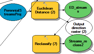
Fig. 6: Modelbuilder process to create a spatial layer for proximity to streams.

A prime farm land spatial layer was created by converting farm land feature class to a raster then reclassifying farmland based on their credentials as "prime" (Table 2)(Fig. 7).

Fig. 7: ModelBuilder process for creating farm land spatial layer.

The third spatial layer was created to find distance from residential areas as noise pollution, air pollution, and traffic can be a concern for residents living near by. Euclidean Distance was used to find proximity to residential zones in a zonation feature class and the result was reclassified to rank closer proximity as high impact areas (Table 2) (Fig. 8).

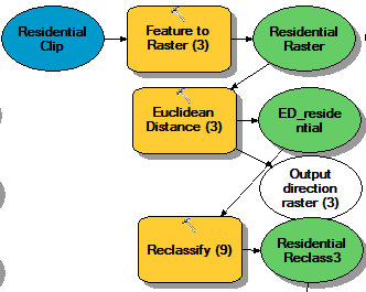
Fig. 8; ModelBuilder process to create a spatial layer for proximity to residential areas.

School districts were not included in residential zones and may also be impacted by the effects of noise and air pollution as well as traffic. I created a spatial layer to find proximity from school districts by first creating an SQL statement to find all land parcels that were owned by a school district. I then used Euclidean Distance and Reclassify to find proximity and rank the areas closest to school districts as high impact areas (Table 2) (Fig. 9).

Fig. 9: ModelBuilder process to find proximity from schools and rank areas within close proximity to schools as high impact regions.

The last spatial layer looked at proximity to Wildlife areas because the noise and air pollution can affect the animals within these designated regions and can be considered a nuisance to anyone hiking or exploring these areas. Euclidean Distance was used to find proximity and Reclassify was used to rank areas closest to wildlife regions as high impact areas (Table 2) (Fig. 10).

Fig. 10: ModelBuilder process to designate close proximity to Wildlife areas
as high impact and areas farther from Wildlife areas as low impact regions.

An environmental and community risk model was created using Raster Calculator by multiplying all 5 spatial layers with a mathematical expression. High values indicate high risk areas. To further examine any impacts, a viewshed was created to determine if any possible mine locations could be seen from an area of importance of value. I chose High Cliff Park as it is a tourist destination for its beauty and outdoor recreation. I converted the polygon border of High Cliff Park to a Raster then converted this Raster to Point Data with the center of the polygon expressed as a point. I then added this into the Viewshed tool and used the suitability model as locations of interest (Fig. 11).

Fig. 11: Using Viewshed to determine if suitable mine locations could be seen from High Cliff Park.

I then reclassified the environmental risk model and the suitability model and combined these outputs to find a model for the best locations suited for frac sand mines (Fig. 12).  The entire process can be seen in Figure 13. I also used PyScripter to create a Best Locations model in which streams were more important than all other factors. The script can be seen under "Script 3" in my Python Scripts page.

Fig. 12: ModelBuilder process to reclass and combine suitable land and environmental risk models into a model displaying the best locations for frac sand mines.

Fig. 13: Creating a suitability model and environmental and community risk model in one flow model in ModelBuilder.

Results

Land Suitability Criteria Spatial Layers Output

Spatial Layer outputs from the model builder process used to create a Suitability Model for suitable frac sand mine land. Criteria include proper geology, Land Cover (excluding completely unusable land such as the types with standing water), Land Cover Type, proximity to rail terminals, gentle slopes, and water table depth. Figure 14 shows all outputs, Table 1 is shown below again to reference values.

A complete Suitability Model displays the suitability of the land in the study area within Trempealeau County, Wisconsin. This was created by a raster calculator mathematical expression in which all land suitability criteria spatial layers were multiplied together (Fig. 15).

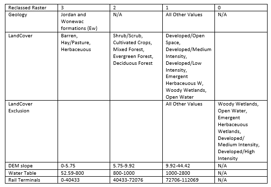
Table 1: Reclassification of Suitability Criteria Spatial Layers where 3= Most Suitable, 2= Medium Suitability, 1= Low Suitability, and 0= Exclusion.

Fig. 14: Land Suitability Criteria outputs for Frac Sand Mine Locations in Trempealeau County, Wisconsin.

Fig. 15: Completed Suitability Model created from all 6 Suitable Land spatial layer criteria.

Potential Environmental and Community Impacts Spatial Layer Outputs

Spatial layers output for criteria for potential environmental and community impacts associated with frac sand mining. Criteria include potential impacts on perennial streams, prime farmland, residential zones, school districts, and wildlife zones. All potential impacts are taken from proximity measurements from the criteria as they are all important environmental and community aspects. Figure 16 shows all spatial layer outputs and Table 2 is shown again for reference of distance rankings for each criterion.

A complete Environmental and Community Risk Model was created in raster calculator with a mathematical expression multiplying all 5 criteria (Fig. 17).

Table 2: Reclassifications of values for each spatial layer used to create an Environmental and Community Risk Model where 3= high impact, 2= medium impact, and 1= low impact.

Fig. 16: All 5 environmental and community criteria that are potentially impacted by Frac Sand Mines. Maps display low, medium, and high potential impacts for each of the 5 criteria.

Fig. 17: Environmental and Community Risk Model using all 5 spatial layers created from the 

environmental and community criteria.

Best Locations


The Suitability Model and the Environmental and Community Risk model were combined to create an index of Best Locations to place potential future Frac Sand Mines in Trempealeau County, Wisconsin (Fig. 18).

Fig. 18: Best Frac Sand Mine Locations with the least environmental and community impacts and most suitable land criteria where 1=least optimal and 6= most optimal. 

Viewshed Analysis

Suitable mine locations viewable from Hill Cliff Park (Fig. 19).

Fig. 19: Suitable mine locations able to be seen from Hill Cliff Park. 

Discussion

The suitability model shows much of the suitable lands for potential future frac sand mines are within the middle to northern portion of Trempealeau County. These are areas that contain ideal sandstone types, exclude all wetland and areas with standing water, areas with more gentler slopes, and areas in which the water table is relatively closer to the land surface. 

The risk model shows that much of the area in Trempealeau County is a risk to environmental and community factors. There are only small areas of land in which frac sand mines would not be as much a risk to residential zones, school districts, wildlife zones, prime farmland, and perennial streams. 

The Best Locations index shows areas of Trempealeau county with the least amount of environmental and community impacts and the highest level of land suiability given all of the criteria investigated during this activity. Much of the land in Trempealeau County is ill-advised for use for frac sand mines. It would be advised to only build future frac sand mines in the designated locations mapped in Figure 18 with the highest ranking.

According to the viewshed analysis, much of the suitable mine locations are within view from Hill Cliff Park, a popular tourist attraction in Trempealeau County. Some of the least suitable land for mines is out of sight from Hill Cliff Park. This makes building frac sand mines in suitable locations difficult if it is of high importance to hide it from sight from Hill Cliff Park.

Conclusion

During this activity, I created multiple spatial layers in ModelBuilder by utilizing conversion and spatial anylist tools. I was able to created suitability and risk models as well as a combined suitability and risk index for frac sand mine locations utilizing raster calculator in map algebra tools and even experimented with viewshed to see if potential best locations for mines could be seen from a popular park attraction. This activity was important for practicing setting up risk and suitability assessments that can be used for future projects such as estimating potential threats to an endangered species or finding best locations for structures designed to boost ecosystem biodiversity. 

Sources:

For Travel Information and Parks in Trempealeau County: http://www.travelwisconsin.com/southwest/trempealeau-county/galesville

Trempealeau County Land Record's Division Website for Water Table Elevation Data: https://wgnhs.uwex.edu/pubs/000444/

Network Analysis

Objective:

Road damage caused by transport of sand via trucks from mines to rail terminals is a concern many Wisconsin communities have. The weight from these trucks can have impacts on the amount and frequency of road maintenance necessary to keep the roads safe for travelers which influences the dollar amount communities pay for this maintenance. Although some costs of road maintenance can be lessened through agreements between county governments and mining companies such as the Road Upgrade Maintenence Agreement (RUMA), it is critical to understand the base impact these mining companies could have on the road systems. In 2013, it was estimated that each year, mining companies in Wisconsin would transport 40 million tons of frac sand out of Wisconsin via trucks and rail cars (Hart, Adams, and Schwartz, 2013). This would undoubtedly heavily impact roadways for county residents as much of this sand would be trucked via rural roadways to railways. The video below shows a 40-minute time lapse of trucks transporting sand to and from a mine near Bloomer, Wisconsin and demonstrates just how much sand is transported from these sand mines.

Some costs can be mitigated by locating which routes would be the most efficient route between mines and rail terminals for the trucks to transport the frac sand. Utilizing Network Analysis tools is a great way to investigate and plan these efficient routes.

The objective of this lab was to introduce Network Analysis as a means of logistical planning. In this lab, I utilize python scripter to prepare our data from ESRI street map USA and the mine locations from the DNR mentioned in the previous geocoding activity. I use network analysis tools in model builder to find the most efficient routes between mines and rail terminals in terms of distance and to calculate a hypothetical cost to each county with data set arbitrarily by our professor.

Methods

Preparing Data Using Python

I began this lab by preparing the ESRI street map data in PyScripter. Through this script, I write and run SQL statements to select all active mines that have the word "mine" and lack the word "rail" in the facility type. This selection contains only the mines that are currently active, are the mine portion of the company, and lack a rail terminal within the mine facility, thus having a potential impact on local roads. After creating feature layers from these selections, I select mines within the state of Wisconsin and remove mines that are within 1.5km of a railway. More information on the script and a screen shot of the script itself can be found in my Python Script page listed as "Python Scripting Activity II: Network Analysis Data Preparation" (here).

Calculating Routes Using the Closest Facility Tool

I imported the python script feature class result (mines within Wisconsin that are 1.5km away from rail terminals), ESRI street map data that consisted of a network of streets, rail terminals to begin calculating routes between mine facilities and rail terminals. Using the Closest Facility tool in the Network Analysis toolbar, I loaded the locations with the rail terminals as the facilities and the mines as the incidents. I then solved the to find the closest rail terminal to each mine. The tool successfully resulted with each of the 44 mines (incidents) and their closest rail terminal (facilities) correctly located (Fig. 1) with a route calculated between each mine and its closest rail terminal (Fig. 2).

Fig. 1: Screenshot of the Network Analyst Window showing result of the Closest Facility Tool.

Fig. 2: Result of the Closest Facility Tool in the Network Analysis toobar displaying routes between each mine and its closest rail terminal.

Using Model Builder to Calculate Hypothetical Costs

After utilizing the Network Analysis Toolbar to calculate the closest facilities and most efficient routes, I began using model builder to estimate the distance traveled in each county by frac sand trucks and to estimate the cost of road maintenance for each county using the hypothetical data given to the class by the professor for number of trucks, for each route and the cost per mile for road maintenance.

I started model builder with rerunning the Closest Facility tool to recalculate routes merely for practice in model builder (Fig. 3). This step was unnecessary as the results from the Closest Facility tool had already been exported into the map as feature classes for facility, incidents, and routes. However, it was good measure to compare the results from the previous run of the Closest Facility tool and the results from the model builder. The resulting incidents, facilities, and routes from the model builder was consistent with the manual Closest Facility tool results.

To calculate closest facilities in Model Builder, I added the Make Closest Facility Layer tool with the ESRI street data as the input. I then specified my mines feature class as incidents by adding the Add Location tool. I added another Add locations tool to specify my rail terminal feature class as the facilities. The Solve tool was added to solve the closest facility tool and calculate routes.
After generating closest facilities, I added the Select Data tool to select route data from the closest facility output. I then added the Copy Features tool to create this selected route data a new feature class which I appropriately named "Routes." I projected the outcome to NAD 1983 UTM Zone 15N to match the rest of the data layer using the Project tool.

Fig. 3: Model Builder process for calculating routes and projecting the resulting routes feature class into an appropriate projection.

From here, I started the process of calculating the distance traveled and hypothetical costs per county. I began by projecting the county boundaries feature class into the same projection as the previous outputs and intersecting this result with the projected routes feature class (Fig. 4).

Fig. 4: Projecting and intersecting the county boundary feature class with the projected routes feature class in Model Builder.

I then used the Summary Statistics tool to calculate the total length of the routes per county. From this result, I used the Add Field tool to add a field called "Dist_miles" in which I would then calculate, using the Calculate Field tool, the total distance traveled, in miles, in each county (Fig. 5). The expression used to calculate this field was the sum of the shape length from the previous summary result * 50 (trucks) * 2 (each truck traveled to and from the rail terminals) * 0.000621371 (conversion from meters to miles) (Fig. 6).

Fig. 5: Summarizing route length, adding distance field, and calculating the distance field in Model Builder.

Fig. 7: Calculate Field window displaying calculation expression for distance traveled per county.

To calculate the cost, I added another Summary Statistics tool to the intersect output to summarize route length by county, just as I had done before adding the distance field. I used the Add Field tool again to add a field for cost, titled "Cost." Finally, I calculated the field with the expression as the [SUM_Shape_Length] * 50 * 2 * 0.000621371 * 2.2 / 100 with the (2.2/100) sequence representing the 2.2 cents it hypothetically costed to maintain a mile of road length. The final Model Builder process can be seen in Figure 8.

Fig. 8: The full Model Builder process.

Results

The result of the Calculate Field tool for distance yielded an attribute table with the Distance in miles field containing values of total miles traveled by frac sand trucks to and from mines and rail ways in each county (Fig. 9). I displayed the distance in a bar graph created in ArcMap (Fig. 10). The Calculate Field tool appropriately calculated the cost per county for the distance traveled by frac sand trucks within the area and the result is displayed in an attribute table (Fig. 11) and in a graph created in ArcMap (Fig.12).

Fig. 9: Distance in miles listed as "Dist_miles" field in the Model Builder output.

Fig. 10: Distance Traveled in each county.

Fig. 11: Cost per county listed as the "Cost" field in the Model Builder output.

Fig. 12: Cost per county.

Each county varied greatly in hypothetical potential cost in road maintenance. Some counties, such as Buffalo and Pepin would only pay between $2.80 and $27.11 while other counties, like Chippewa and Eau Claire would need to pay between$277.67-$613.61 (Fig. 13).

Fig. 13: Final map depicting the costs for road maintenance by county.

Discussion

In Fig. 12, you can see that the counties with the highest hypothetical cost for road maintenance are Chippewa ($613.14), Eau Claire ($385.22), and Barron ($371.72). If this data were taken from a real data set for number of trucks and the cost for road maintenance, these counties would need to be aware of the impact the mining companies have on their local roads and may want to consider an agreement plan between mining companies and the government much like RUMA. However, all counties containing mine to rail routes should be aware of potential impacts on their road maintenance. At the beginning of the lab, before I had removed rail terminals outside of Wisconsin, I noticed there were a couple terminals that may be even closer to some of the mines along the border of Wisconsin. If I were to do the lab again, it may be wise to keep rail terminals in Minnesota and Wisconsin to see if there could be a more efficient way to transport the sand. However, this would have potential to raise issues between the two states. Because the closest Wisconsin rail terminal to the mine located in Burnett County has a most efficient route through the state of Minnesota, this may already be a problem without considering rail terminals in Minnesota for closest facilities (Fig. 13). 

 Conclusion

In this lab, we used PyScripter to set up queries and create feature layers and used Network Analysis tools in the Network Analysis toolbar as well as in Model Builder to calculate the closest facilities and most efficient routes as well as hypothetical distances traveled and cost of road maintenance per county due to frac sand trucking. These Network Analysis tools can be and are currently used by many businesses to plan logistics for shipping products. For this lab, however, since our data was only hypothetical, I cannot derive any true conclusion about frac sand transport and the most efficient routes and costs to counties. Though this is a useful skill that other businesses and research projects may require.

Sources

Hart, M. V., Adams, T. & Schwartz, A. (2013). Transportation Impacts of Frac Sand Mining in the MAFC Region: Chippewa County Case Study. In Mid-America Freight Coalition. Retrieved: November 19, 2013, From http://midamericafreight.org/wp-content/uploads/FracSandWhitePaperDRAFT.pdf. 

Data Normalization, Geocoding, and Error Assessment for Mines in Wisconsin

Objective

Upon being given addresses for several sand mines in Wisconsin from the DNR, the goal of this lab was to be able to normalize the data table of addresses, geocode the mine locations to a map, and check for error by comparing the geocoded locations with other classmates and the DNR's geocoded locations. Because not all addresses were given in the same format, we used different methods to geocode the mines. One big difference was between finding mine locations with street addresses versus locating mines with PLSS addresses. 

Methods

The first step in geocoding the mines was to normalize the data table of addresses. To do this, first gathered all the addresses that I was assigned to from a master list of addresses. I then separated all address elements such as PLSS, Street Name, City, and State into separate columns.This was necessary for ArcMap to be able to appropriately and more accurately locate the mine addresses by matching the elements of the locations separately. The Figures below show the original format of the table containing all addresses (Fig. 1) and the format of the table containing the addresses for this lab (Fig. 2). Note the "Address" attribute of the original table is broken into "PLSS," and "Road," and the "Town/City/Village," is separated into "Town," and "City" attributes in the normalized table.

Fig. 1: Original format of the address data table before normalization.

Fig. 2: Data table format of addresses after normalization. 

After normalizing the table, I then imported my table to ArcMap to begin gecoding using the Geocode Addresses tool and World Geocode Service as an Address Locator. When the Geocode Addresses tool was finished matching addresses from the table to the map, I used the Review/Rematch Addresses tool on the geocoding toolbar to determine the accuracy of the matches. I used status and score to determine if I needed to manually geocode an address. If the status was "Tied" or "Unmatched," I needed to locate the address manually and use "Pick Address From Map" to create a match for that mine (Fig. 3). I would not accept any match score below 90%, though it was only necessary to accept matches above 85%. This ensured a greater accuracy of the data. Several addresses were unmatched and tied at the start of the review/rematch process and two locations were matched with low scores. For matches below 90% score and "Tied" or "Unmatched," I used google earth to type in the address of the mine and show me the area where the mine should theoretically be and to help locate the mine on the basemap on ArcMap. For PLSS locations, I used the PLSS data from WiDNR2014 database and an SQL for PLSS name to locate the area in which the mine resided. I then searched the PLSS area to find the mine and then used "Pick Address From Map" to create a match for the mine location. I did this until all mine locations were matched with a score above 90% (Fig. 4). All locations were matched with a score of 100% save for one location automatically matched at 94.61%.

Fig.3: An example of a matched mine location . The address location is symbolized by the green dot at the beginning of the driveway of the mine.

Fig. 4: Review/Rematch Interactive Window showing completed Review/Rematch process with a 100% match rate.

After editing the mine locations in the Review/Rematch interactive session, I exported my mine locations as a shapefile and uploaded them to a shared folder for my classmates to compare locations with. I then uploaded my classmates shapefiles and the geocoded locations from the DNR and brought them into ArcMap. I merged the files of my classmates and my mine location file using the Merge tool in Data Management and left the DNR mine location file unaltered to compare my locations with the DNR and the class separately. I then wrote an SQL expression to select out the Mine Unique ID's that matched the Mine Unique ID's I had previously geocoded (Fig. 5). I saved the SQL expression to be able to load it into another SQL window easily instead of typing it again. Since the expression was lengthy, this saved much time. After selecting the similar Mine ID locations, I created a new layer from the selected features for both the DNR's actual locations and my geocoded mine locations.

Fig. 5: SQL Expression to select Mine Unique ID's that were the same as the Mine Unique ID's I had previously geocoded.

I then used the Generate Near Table tool to calculate the distance between the points in my mine locations and my classmates locations(Fig. 6) and between my mine locations and the actual locations from the DNR (Fig. 7). To find the amount of average error, I summarized the table's near distance attribute to get an average distance between the locations of each feature class. This is discussed in the Results section.

Results

8 of the geocoded mine locations matched perfectly with the geocoded mines of my classmates while only 5 of my geocoded mine locations matched the actual mine locations given by the DNR (tables in Fig. 6 and 7). The summary of distance showed an average distance between my mine locations and the classmates was 0.012048 and an average distance between my mine locations and the actual locations was 0.036308. I was closer to my classmate's geocoded locations than the actual locations given to us by the DNR. 

Fig.6: Distance between my mine locations and my classmates.

Fig. 7: Distance between my mine locations and their actual locations from the DNR.

Discussion

There are many reasons for spatial discrepancies in geocoding processes. Below is a table of error types and examples from Lo, chapter 4 (Fig. 8). In this geocoding lab, I experienced many operational errors such as field measurement confusion on which driveway to match to the address when there were multiple driveways for one mine. One example of inherent error that may be an influence on the spatial differences between geocoded mines and the actual locations is the aging of the map. Frac Sand Mining is a rapidly growing business and satellite imagery is not able to keep up. In some instances, mines could not be found in their supposed location and an estimate had to be made.

Fig. 8: Error types and examples from Lo chapter 4.

One way to know which geocoded points are correct is to rank the points and give more weight to those that have come from a reputable source, such as the DNR. You can also check the points across multiple sources of data such as we did in this lab when comparing geocoded mines with classmates. 

Conclusion

Geocoding can be an important step in spatial studies as it allows you to locate addresses that have not yet been added to a map. In a study such as the frac sand mining study we will be continuing with this semester, geocoding is needed when the industry is growing at a fast rate. I now have a greater sense for the importance of table normalization and obtaining accurate data. After completing this lab, we now have the locations of mines in Wisconsin to continue our study on Frac Sand Mining in Western Wisconsin. 

Data Gathering

Objectives

The goal of this assignment was to become familiar with the process of downloading data from different sources on the internet then organizing and preparing the data for use in ArcGIS. This included joining some data, projecting all data from different sources into a common coordinate system and building a geodatabase in which to store and organize the newly prepared data. Since focus is given to Trempealeau County, a Python script was written to clip all data to the border of this county which you can read more about here.

The data collected from this exercise will be used for later activities this semester in exploring issues surrounding sand mining and creating a suitability and risk model for sand mining in Tremplealeau County.

Methods

Data on sand frac mining in Trempealeau County, Wisconsin was collected by first downloading zip files and extracting them to a working folder. Then, using Python Scripting, the data was projected into a common coordinate system, clipped to the Trempealeau County border, and extracted. A geodatabase was built and the projected and clipped data was then loaded into it and extra, redundant data was deleted to better organize the data. This can be summarized by the data flow model taken from our exercise instructions sheet below (Fig. 1). The final step was to create metadata for the downloaded data to assess data accuracy.

Figure 1: Data flow model depicting the process of downloading data from different sources and preparing them for use in ArcGIS.

Step One: Downloading Data From Various Internet Sources

Data was first gathered from different internet sources by navigating source sites and downloading zip files of the data of interest. The data zip files and the sources from which they were obtained are listed below:

1. USDT NTAD Railway Network at http://www.rita.dot.gov/bts/sites/rita.dot.gov.bts/files/publications/national_transportation_atlas_database/2015/polyline

2. USGS Elevation Data at http://nationalmap.gov/about.html

3. USDA National Land Use Data at http://datagateway.nrcs.usda.gov/

4. Trempealeau County land records Trempealeau County Geodatabase at http://www.tremplocounty.com/landrecords/

5. USDA NRCS Web Soil Survey SSURGO data at http://websoilsurvey.sc.egov.usda.gov/App/HomePage.htm


Once the data were downloaded as zip files into a temporary folder, I extracted the data from the zip files into a working file. I then separated raster data in .tif form for the elevation data, railroads, soils, land use, and croplands into a newly created geodatabase to be processed.


Step Two: Using Python Scripting to Process the Data and Load into a New Geodatabase 

I created a python script in Python Script Editor (found here) to project the raster files into the same coordinate system as the data in the Trempealeau County Geodatabase and clip the data by the county boundary and save the new data in the newly created geodatabase (Fig.2). After this was completed, I then created maps depicting the elevation data, croplands, and land use (seen in the results section) (Fig. 3-5).

Figure 2: Python Script used for processing.

Step Three: Deleting Redundant Data

After all data was downloaded, organized, extracted, processed, and saved into a single geodatabase, it was important to delete redundant data to free space in the computer storage and ensure proper organization. For this reason, I created a metadata table for the data downloaded. The table includes scale, effective resolution, minimum mapping unit, planimetric coordinate accuracy, lineage, and temporal and attribute accuracy. The finished table can be seen in the results section (Fig.6).

Step Four: Creating Metadata for Data Accuracy

Because the data in this exercise was collected from multiple sources and will be used later to investigate issues surrounding sand frac mining in western Wisconsin, it is important to keep a record of metadata of all data to ensure accuracy of future analysis.

Results

The figures below show the maps of Trempealeau County elevation, croplands, and land use after downloading, projecting, clipping data from various sources (Fig. 3-5). The finished metadata can also be seen below (Fig. 6).

Maps

Figure 3-5: 3) (left) Digital elevation model of Trempealeau County from USGS, 4) (middle) Croplands/Agriculture in Trempealeau County from USDA, 5) (right) Land Use in Trempealeau County from USDA/NASS.

Metadata

Figure 6: Metadata of downloaded data. "NA" indicates the areas I was unable to find.

Conclusion

Successfully downloading, organizing, and processing data as well as locating and understanding metadata and data accuracy is a critical part of any project using geospatial information systems. In this lab, we gained exposure to these processes, using python scripting to complete the processing portion of this activity which included projecting and clipping to the Trempealeau County border. This lab's data collection, processing and metadata and data accuracy results are valuable for future analysis that will take place in this semester's project in assessing suitability and risk of frac sand mining in Trempealeau County.