Network Analysis

Objective:

Road damage caused by transport of sand via trucks from mines to rail terminals is a concern many Wisconsin communities have. The weight from these trucks can have impacts on the amount and frequency of road maintenance necessary to keep the roads safe for travelers which influences the dollar amount communities pay for this maintenance. Although some costs of road maintenance can be lessened through agreements between county governments and mining companies such as the Road Upgrade Maintenence Agreement (RUMA), it is critical to understand the base impact these mining companies could have on the road systems. In 2013, it was estimated that each year, mining companies in Wisconsin would transport 40 million tons of frac sand out of Wisconsin via trucks and rail cars (Hart, Adams, and Schwartz, 2013). This would undoubtedly heavily impact roadways for county residents as much of this sand would be trucked via rural roadways to railways. The video below shows a 40-minute time lapse of trucks transporting sand to and from a mine near Bloomer, Wisconsin and demonstrates just how much sand is transported from these sand mines.

Some costs can be mitigated by locating which routes would be the most efficient route between mines and rail terminals for the trucks to transport the frac sand. Utilizing Network Analysis tools is a great way to investigate and plan these efficient routes.

The objective of this lab was to introduce Network Analysis as a means of logistical planning. In this lab, I utilize python scripter to prepare our data from ESRI street map USA and the mine locations from the DNR mentioned in the previous geocoding activity. I use network analysis tools in model builder to find the most efficient routes between mines and rail terminals in terms of distance and to calculate a hypothetical cost to each county with data set arbitrarily by our professor.

Methods

Preparing Data Using Python

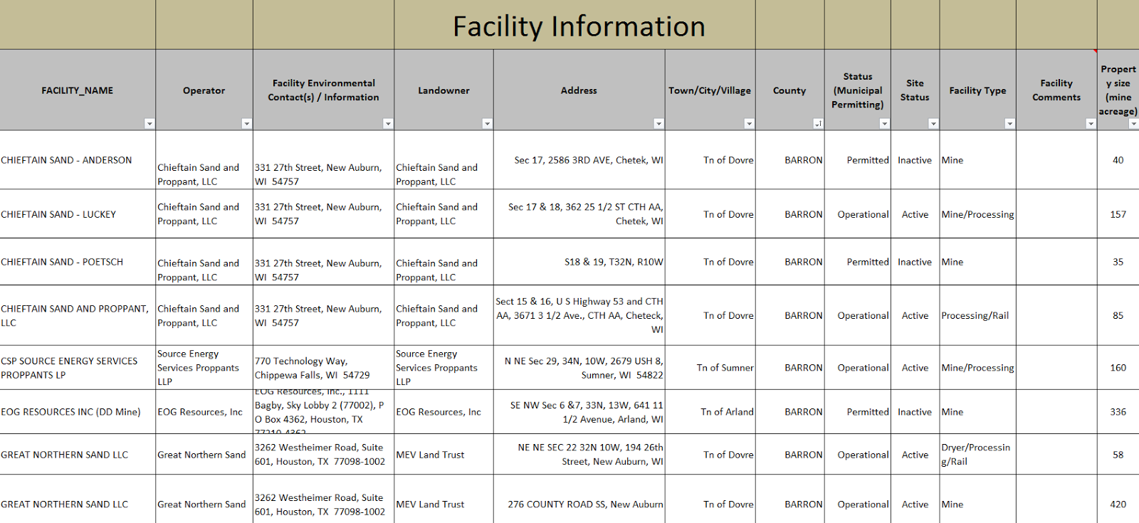
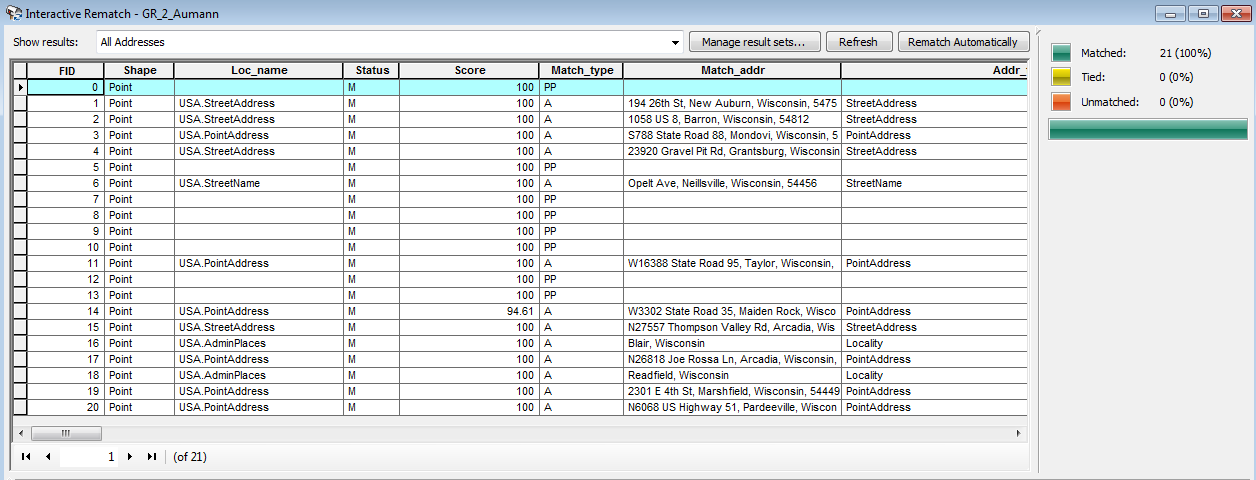
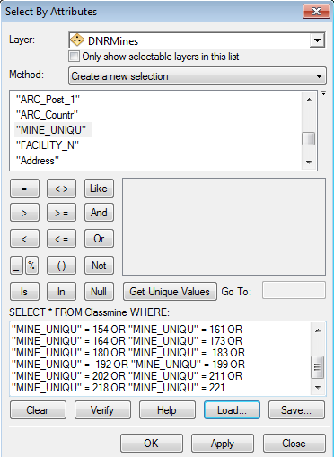
I began this lab by preparing the ESRI street map data in PyScripter. Through this script, I write and run SQL statements to select all active mines that have the word "mine" and lack the word "rail" in the facility type. This selection contains only the mines that are currently active, are the mine portion of the company, and lack a rail terminal within the mine facility, thus having a potential impact on local roads. After creating feature layers from these selections, I select mines within the state of Wisconsin and remove mines that are within 1.5km of a railway. More information on the script and a screen shot of the script itself can be found in my Python Script page listed as "Python Scripting Activity II: Network Analysis Data Preparation" (here).

Calculating Routes Using the Closest Facility Tool

I imported the python script feature class result (mines within Wisconsin that are 1.5km away from rail terminals), ESRI street map data that consisted of a network of streets, rail terminals to begin calculating routes between mine facilities and rail terminals. Using the Closest Facility tool in the Network Analysis toolbar, I loaded the locations with the rail terminals as the facilities and the mines as the incidents. I then solved the to find the closest rail terminal to each mine. The tool successfully resulted with each of the 44 mines (incidents) and their closest rail terminal (facilities) correctly located (Fig. 1) with a route calculated between each mine and its closest rail terminal (Fig. 2).

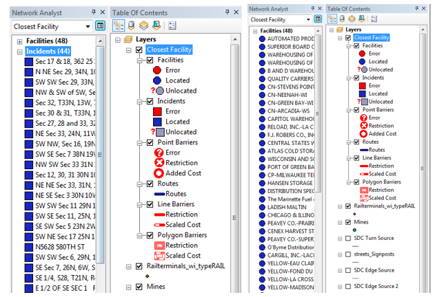Fig. 1: Screenshot of the Network Analyst Window showing result of the Closest Facility Tool.

Fig. 2: Result of the Closest Facility Tool in the Network Analysis toobar displaying routes between each mine and its closest rail terminal.

Using Model Builder to Calculate Hypothetical Costs

After utilizing the Network Analysis Toolbar to calculate the closest facilities and most efficient routes, I began using model builder to estimate the distance traveled in each county by frac sand trucks and to estimate the cost of road maintenance for each county using the hypothetical data given to the class by the professor for number of trucks, for each route and the cost per mile for road maintenance.

I started model builder with rerunning the Closest Facility tool to recalculate routes merely for practice in model builder (Fig. 3). This step was unnecessary as the results from the Closest Facility tool had already been exported into the map as feature classes for facility, incidents, and routes. However, it was good measure to compare the results from the previous run of the Closest Facility tool and the results from the model builder. The resulting incidents, facilities, and routes from the model builder was consistent with the manual Closest Facility tool results.

To calculate closest facilities in Model Builder, I added the Make Closest Facility Layer tool with the ESRI street data as the input. I then specified my mines feature class as incidents by adding the Add Location tool. I added another Add locations tool to specify my rail terminal feature class as the facilities. The Solve tool was added to solve the closest facility tool and calculate routes.
After generating closest facilities, I added the Select Data tool to select route data from the closest facility output. I then added the Copy Features tool to create this selected route data a new feature class which I appropriately named "Routes." I projected the outcome to NAD 1983 UTM Zone 15N to match the rest of the data layer using the Project tool.

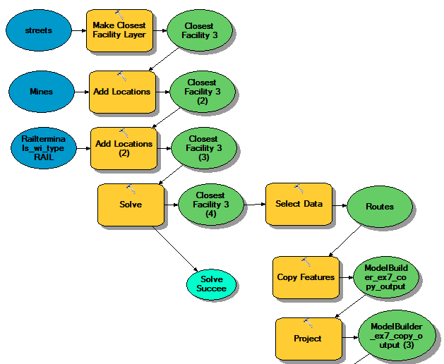Fig. 3: Model Builder process for calculating routes and projecting the resulting routes feature class into an appropriate projection.

From here, I started the process of calculating the distance traveled and hypothetical costs per county. I began by projecting the county boundaries feature class into the same projection as the previous outputs and intersecting this result with the projected routes feature class (Fig. 4).

Fig. 4: Projecting and intersecting the county boundary feature class with the projected routes feature class in Model Builder.

I then used the Summary Statistics tool to calculate the total length of the routes per county. From this result, I used the Add Field tool to add a field called "Dist_miles" in which I would then calculate, using the Calculate Field tool, the total distance traveled, in miles, in each county (Fig. 5). The expression used to calculate this field was the sum of the shape length from the previous summary result * 50 (trucks) * 2 (each truck traveled to and from the rail terminals) * 0.000621371 (conversion from meters to miles) (Fig. 6).

Fig. 5: Summarizing route length, adding distance field, and calculating the distance field in Model Builder.

Fig. 7: Calculate Field window displaying calculation expression for distance traveled per county.

To calculate the cost, I added another Summary Statistics tool to the intersect output to summarize route length by county, just as I had done before adding the distance field. I used the Add Field tool again to add a field for cost, titled "Cost." Finally, I calculated the field with the expression as the [SUM_Shape_Length] * 50 * 2 * 0.000621371 * 2.2 / 100 with the (2.2/100) sequence representing the 2.2 cents it hypothetically costed to maintain a mile of road length. The final Model Builder process can be seen in Figure 8.

Fig. 8: The full Model Builder process.

Results

The result of the Calculate Field tool for distance yielded an attribute table with the Distance in miles field containing values of total miles traveled by frac sand trucks to and from mines and rail ways in each county (Fig. 9). I displayed the distance in a bar graph created in ArcMap (Fig. 10). The Calculate Field tool appropriately calculated the cost per county for the distance traveled by frac sand trucks within the area and the result is displayed in an attribute table (Fig. 11) and in a graph created in ArcMap (Fig.12).

Fig. 9: Distance in miles listed as "Dist_miles" field in the Model Builder output.

Fig. 10: Distance Traveled in each county.

Fig. 11: Cost per county listed as the "Cost" field in the Model Builder output.

Fig. 12: Cost per county.

Each county varied greatly in hypothetical potential cost in road maintenance. Some counties, such as Buffalo and Pepin would only pay between $2.80 and $27.11 while other counties, like Chippewa and Eau Claire would need to pay between$277.67-$613.61 (Fig. 13).

Fig. 13: Final map depicting the costs for road maintenance by county.

Discussion

In Fig. 12, you can see that the counties with the highest hypothetical cost for road maintenance are Chippewa ($613.14), Eau Claire ($385.22), and Barron ($371.72). If this data were taken from a real data set for number of trucks and the cost for road maintenance, these counties would need to be aware of the impact the mining companies have on their local roads and may want to consider an agreement plan between mining companies and the government much like RUMA. However, all counties containing mine to rail routes should be aware of potential impacts on their road maintenance. At the beginning of the lab, before I had removed rail terminals outside of Wisconsin, I noticed there were a couple terminals that may be even closer to some of the mines along the border of Wisconsin. If I were to do the lab again, it may be wise to keep rail terminals in Minnesota and Wisconsin to see if there could be a more efficient way to transport the sand. However, this would have potential to raise issues between the two states. Because the closest Wisconsin rail terminal to the mine located in Burnett County has a most efficient route through the state of Minnesota, this may already be a problem without considering rail terminals in Minnesota for closest facilities (Fig. 13). 

 Conclusion

In this lab, we used PyScripter to set up queries and create feature layers and used Network Analysis tools in the Network Analysis toolbar as well as in Model Builder to calculate the closest facilities and most efficient routes as well as hypothetical distances traveled and cost of road maintenance per county due to frac sand trucking. These Network Analysis tools can be and are currently used by many businesses to plan logistics for shipping products. For this lab, however, since our data was only hypothetical, I cannot derive any true conclusion about frac sand transport and the most efficient routes and costs to counties. Though this is a useful skill that other businesses and research projects may require.

Sources

Hart, M. V., Adams, T. & Schwartz, A. (2013). Transportation Impacts of Frac Sand Mining in the MAFC Region: Chippewa County Case Study. In Mid-America Freight Coalition. Retrieved: November 19, 2013, From http://midamericafreight.org/wp-content/uploads/FracSandWhitePaperDRAFT.pdf. 

Data Normalization, Geocoding, and Error Assessment for Mines in Wisconsin

Objective

Upon being given addresses for several sand mines in Wisconsin from the DNR, the goal of this lab was to be able to normalize the data table of addresses, geocode the mine locations to a map, and check for error by comparing the geocoded locations with other classmates and the DNR's geocoded locations. Because not all addresses were given in the same format, we used different methods to geocode the mines. One big difference was between finding mine locations with street addresses versus locating mines with PLSS addresses. 

Methods

The first step in geocoding the mines was to normalize the data table of addresses. To do this, first gathered all the addresses that I was assigned to from a master list of addresses. I then separated all address elements such as PLSS, Street Name, City, and State into separate columns.This was necessary for ArcMap to be able to appropriately and more accurately locate the mine addresses by matching the elements of the locations separately. The Figures below show the original format of the table containing all addresses (Fig. 1) and the format of the table containing the addresses for this lab (Fig. 2). Note the "Address" attribute of the original table is broken into "PLSS," and "Road," and the "Town/City/Village," is separated into "Town," and "City" attributes in the normalized table.

Fig. 1: Original format of the address data table before normalization.

Fig. 2: Data table format of addresses after normalization. 

After normalizing the table, I then imported my table to ArcMap to begin gecoding using the Geocode Addresses tool and World Geocode Service as an Address Locator. When the Geocode Addresses tool was finished matching addresses from the table to the map, I used the Review/Rematch Addresses tool on the geocoding toolbar to determine the accuracy of the matches. I used status and score to determine if I needed to manually geocode an address. If the status was "Tied" or "Unmatched," I needed to locate the address manually and use "Pick Address From Map" to create a match for that mine (Fig. 3). I would not accept any match score below 90%, though it was only necessary to accept matches above 85%. This ensured a greater accuracy of the data. Several addresses were unmatched and tied at the start of the review/rematch process and two locations were matched with low scores. For matches below 90% score and "Tied" or "Unmatched," I used google earth to type in the address of the mine and show me the area where the mine should theoretically be and to help locate the mine on the basemap on ArcMap. For PLSS locations, I used the PLSS data from WiDNR2014 database and an SQL for PLSS name to locate the area in which the mine resided. I then searched the PLSS area to find the mine and then used "Pick Address From Map" to create a match for the mine location. I did this until all mine locations were matched with a score above 90% (Fig. 4). All locations were matched with a score of 100% save for one location automatically matched at 94.61%.

Fig.3: An example of a matched mine location . The address location is symbolized by the green dot at the beginning of the driveway of the mine.

Fig. 4: Review/Rematch Interactive Window showing completed Review/Rematch process with a 100% match rate.

After editing the mine locations in the Review/Rematch interactive session, I exported my mine locations as a shapefile and uploaded them to a shared folder for my classmates to compare locations with. I then uploaded my classmates shapefiles and the geocoded locations from the DNR and brought them into ArcMap. I merged the files of my classmates and my mine location file using the Merge tool in Data Management and left the DNR mine location file unaltered to compare my locations with the DNR and the class separately. I then wrote an SQL expression to select out the Mine Unique ID's that matched the Mine Unique ID's I had previously geocoded (Fig. 5). I saved the SQL expression to be able to load it into another SQL window easily instead of typing it again. Since the expression was lengthy, this saved much time. After selecting the similar Mine ID locations, I created a new layer from the selected features for both the DNR's actual locations and my geocoded mine locations.

Fig. 5: SQL Expression to select Mine Unique ID's that were the same as the Mine Unique ID's I had previously geocoded.

I then used the Generate Near Table tool to calculate the distance between the points in my mine locations and my classmates locations(Fig. 6) and between my mine locations and the actual locations from the DNR (Fig. 7). To find the amount of average error, I summarized the table's near distance attribute to get an average distance between the locations of each feature class. This is discussed in the Results section.

Results

8 of the geocoded mine locations matched perfectly with the geocoded mines of my classmates while only 5 of my geocoded mine locations matched the actual mine locations given by the DNR (tables in Fig. 6 and 7). The summary of distance showed an average distance between my mine locations and the classmates was 0.012048 and an average distance between my mine locations and the actual locations was 0.036308. I was closer to my classmate's geocoded locations than the actual locations given to us by the DNR. 

Fig.6: Distance between my mine locations and my classmates.

Fig. 7: Distance between my mine locations and their actual locations from the DNR.

Discussion

There are many reasons for spatial discrepancies in geocoding processes. Below is a table of error types and examples from Lo, chapter 4 (Fig. 8). In this geocoding lab, I experienced many operational errors such as field measurement confusion on which driveway to match to the address when there were multiple driveways for one mine. One example of inherent error that may be an influence on the spatial differences between geocoded mines and the actual locations is the aging of the map. Frac Sand Mining is a rapidly growing business and satellite imagery is not able to keep up. In some instances, mines could not be found in their supposed location and an estimate had to be made.

Fig. 8: Error types and examples from Lo chapter 4.

One way to know which geocoded points are correct is to rank the points and give more weight to those that have come from a reputable source, such as the DNR. You can also check the points across multiple sources of data such as we did in this lab when comparing geocoded mines with classmates. 

Conclusion

Geocoding can be an important step in spatial studies as it allows you to locate addresses that have not yet been added to a map. In a study such as the frac sand mining study we will be continuing with this semester, geocoding is needed when the industry is growing at a fast rate. I now have a greater sense for the importance of table normalization and obtaining accurate data. After completing this lab, we now have the locations of mines in Wisconsin to continue our study on Frac Sand Mining in Western Wisconsin.